
What is NAPLES?
OVERVIEW
NAPLES stands for New Algorism for Polymeric Liquids Entangled and Strained, and it is a computer code to simulate dynamics of entangled polymers (and thus, rheology as well). The code has been being developed mainly by Yuichi Masubuchi under collaborations with many other researchers including Napolitan professors (Giuseppe Marrucci, Giovanni Ianniruberto and Francesco Greco), Japanese professors (Hiroshi Watanabe, Takashi Uneyama, Jun-ichi Takimoto, Kiyohito Koyama, Masao Doi, etc.) and researchers in Japanese private sector. Couples of channels have been established for code distribution to public (see the links). It is acknowledged that the development has been supported by several fundings such as JST-PRESTO, JST-CREST, NEDO, JSPS. Specifically, the recent development for multi-scale simulations has been being supported by JST-CREST, "High Performance Computing for Multi-scale and Multi-physics Phenomena". Further detail of the NAPLES code is given below.
- BACKGROUNDS
- PCN MODEL
- TYPICAL EXAMPLES
- REFERENCES
BACKGROUNDS
Polymeric liquids such as molten plastics show viscoelasticity[1]. Under a step deformation, initially the material behaves as solid with elastic response and eventually it flows just as liquid. The characteristic time, beyond which the material flows as liquid, is called as the viscoelastic relaxation time.
It has been known that the viscoelastic property of polymers plays a significant role in polymer processing[2]. For instance, for the injection molding, less elastic material (i.e., a material with shorter relaxation time) is preferable to achieve better transferability, higher processing cycle, and reduction of warpage and deformation of the product. However, an adequate elasticity is also demanded to eliminate burr that is generated by undesirable flows into the gap between molds. The material tuning on elasticity is also important in film blowing, blow molding and foaming where the extrudate needs elasticity to keep its shape after the outlet of extruder.
Since the viscoelasticity of polymers is a result of the Brownian motion of molecules, it is strongly dependent on molecular characteristics, i.e., not only chemistry but also molecular weight, its distribution, long chain branching, blending, etc[1]. For instance, when the polymer is in linear shape and its molecular weight is monodispersed, the viscoelastic relaxation time is in proportional to M3 (M: molecular weight). When the material has a distribution in its molecular weight and/or a long chain branching, no simple rule exists to describe the relaxation time as a function of the molecular characteristics.
On the industrial demands to control the processability of material through viscoelasticity, scientific attempts have been made to develop a method to predict viscoelasticity from molecular architecture. Figure 1 shows the position of such studies (including this specific study) in the polymer industry. Not only for the molecular design of virgin materials but also for the recycled materials, relation between polymer architecture and processability (via viscoelasticity) is a critical issue for polymer processing. Since some methods have been already available even in commercial for the evaluation of processability for a given viscoelasticity, the missing link is the prediction of viscoelasticity from polymer architecture.
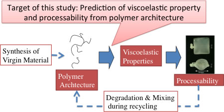
Figure 1 Position of the target of this study in polymer industry.
Remarkable success has been made in molecular theory to predict the viscoelastic properties of polymers but the theory is still under development. Historically (in late 60s’)[3], Edwards pointed out that the entanglement among polymers, which is defined by the motional constraint prohibiting crossing between polymers, generates the elasticity of polymeric liquids. de Gennes and Edwards independently proposed the tube model where the entanglement is replaced by tube shaped motional constraint for single polymer motion. Doi and Edwards derived constitutive equation (which express the viscoelasticity for given molecular weight) for the tube model and showed that some viscoelastic properties can be qualitatively reproduced. The promising results of the Doi-Edwards model lent support the validity of the tube concept, and thus various improvements have been made to achieve further accuracy on the prediction by implementing additional relaxation modes, i.e., contour length fluctuation, constraint release and convective constraint release. For branched polymers, further mechanism has been implemented to take account the relaxation around the branching point. Nevertheless, even by the very recent theories, quantitative prediction for arbitral molecular architecture has never been realized[4]. This is due to the conceptual shortcoming of tube picture in its single chain modeling where the effect of surrounding chains is embedded in the (tube shaped) dynamical constraint for the single chain inside. It is fundamentally difficult to take account the effect of distributions in molecular shape and blending of variety of molecules by the single chain picture.
Another option to predict macroscopic properties from molecular architecture is molecular simulations but the use molecular simulation to viscoelasticity is not practical due to the huge computational cost. To reduce the cost, coarse-grained models have been developed[5]. In the coarse-graining idea, reduction of calculation cost is achieved by introducing a coarse-grained element that represents several atoms. Thus chemistry details of the molecule are somewhat abandoned and the universal nature of polymers such as the entanglement is magnified. For example, Kremer and Grest [5] proposed a typical class of coarse-grained model called bead-spring model, which reasonably reproduces some long time behavior of polymers. Indeed, Likhtman et al [6] reported that the bead-spring model properly predicted the viscoelasticity. In this framework, the effect of molecular architectures including its distribution can be naturally taken account through the many chain nature of the molecular simulation. However, even with the very recent computational power, the viscoelastic calculation for polymers is still infeasible in practical sense. For example, the calculation made by Likhtman et al spent one year CPU time to obtain relaxation of a bead-spring chain system that is roughly comparable to polystyrene melt with the molecular weight of 200,000.
Upon the industrial demands and the state of the art, we have developed a theoretical model called primitive chain network model [7], and a computational code to realize quantitative prediction of viscoelastic properties of variety of polymeric systems. we have constructed the theoretical model utilizing the concept of entanglement to take advantage of its high efficiency in reduction of computational cost. Instead of the single chain modeling used in the conventional tube model, we consider the dynamics of many chains in the sprit of molecular dynamics simulations. Figure 2 shows the position of my model among the conventional methods.
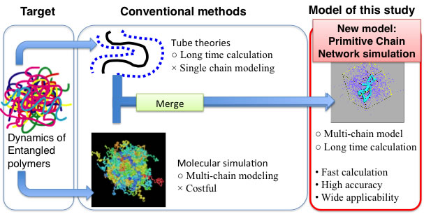
Figure 2 Position of the model developed in this study
The resultant simulation code implementing the primitive chain network model realizes much faster calculation with less cost than the conventional molecular simulations (10,000 times faster than the bead-spring chain calculation at least) with quantitative agreement on viscoelastic properties with experimental data for variety of molecules. 27 original papers (in English) and 8 patents (PCT) have been published, and more than 20 grants have been awarded from the Japanese public funding agencies (JSPS, JST and NEDO) and private companies. Several prizes of scientific societies have been awarded as well, from Rheology Society Japan, Molecular Simulation Society Japan, and Society of Rubber Industry in Japan. The simulation code has been commercially distributed known as NAPLES from the Japanese software companies and the software distributer in US. Details of the model and some typical examples of the simulation shall be presented in the following sections.
PCN MODEL
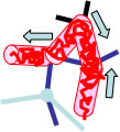
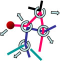
In the PCN model, sliplinks are distributed along the polymer chains to divide them into subchains having a molecular weight comparable to the entanglement molecular weight. Each sliplink bonds two chains, consistently with the binary assumption for entanglements. The sliplink is allowed to move in space according to a balance among drag force, subchain tensions, osmotic force, and random thermal force. The polymer chain slides through the sliplinks (i.e., reptates) to fulfill the force balance along the chain. If the end of the chain moves past a sliplink, that sliplink is removed. On the contrary, if the monomers (taken to be the Kuhn segments) reptate, by a certain amount, beyond the sliplink located at the chain end, a new sliplink is created by hooking one of the surrounding chains. In summary, dynamics of the system is ruled by: 3D motion of the sliplinks, monomer reallocation between adjacent subchains via chain sliding through the sliplinks, and creation/removal of sliplinks at chain ends. Figure 3 schematically shows the PCN model.
Figure 3 Schematic representation of the PCN model
TYPICAL EXAMPLES
Linear viscoelasticity
The viscoelastic response in vicinity of the equilibrium state is called as linear viscoelasticity where the response function under a given flow/deformation history is written by the linear combination of the basic response function. The basic response function is called as the linear relaxation modulus G(t) that is obtained from the auto-correlation function of shear stress under equilibrium, and it is a good measure to characterize viscoelastic material. Usually, G(t) is measured as its Fourier transformed form, G*(w) for the experimental convenience. Thus the prediction of G*(w) is a fundamental test of the model.
Figure 4 Prediction of G*(w) for various polymer melts. Table I Parameters for Fig 4.
In the PCN simulations, the linear viscoelastic response is quantitatively predicted for any kind of polymer architecture and blends. Figure 4 shows the prediction of G*(w) made by PCN simulations for several polymer melts using the parameters in Table I to report quantitative agreement with experiments [8]. It is emphasized that the prediction was made for quite long time range (~104 sec) where the conventional molecular simulations cannot be performed with practical computational cost. As mentioned in the previous section, the parameters were determined by fitting under the relation of G0=rho RT/M0 thus only two parameters (M0 and t0) were tuned. The value of M0 is somewhat close to, but different from the established entanglement molecular weight Me (often tabulated in text books of polymer science) due to the fluctuations taken account in our model [10]. Figure 5 shows G*(w) for mixtures of short and long polymers[9]. Due to the dynamical correlations between in the molecules, G*(w) for mixtures is difficult for prediction by the tube models. For instance, a simple mixing rule does not work for the mixture. On the other hand, according to the multi-chain nature of the PCN model, the dynamical correlation is naturally taken account and thus the predictions are in quantitative agreement. It is emphasized that the parameters are common to Table I, which are obtained for monodispersed melt, and neither further tuning nor addition of parameters is required. Figure 6 shows G*(w) for some branched polymers to report quantitative agreement without any additional parameters to the linear polymer simulation[11-13]. It is noted that there exist a couple of tube theories reporting similar results, but these theories require additional empirical parameters for fitting.
Figure 5 (Left) G*(w) for short and long chain mixtures. The long chain content is 1.0, 0.6, 0.4, 0.2, 0.1 and 0 from left to right.
Figure 6 (Right) G*(w) for H-Branch polymers with the molecular weight of the arm chain Ma and the bridge chain Mb.
Non-linear viscoelasticity
The viscoelastic response under large and fast deformations is categorized as non-linear viscoelasticity where the simple linear relation between relaxation modulus and the response functions is no longer valid. Due to its non-linear nature, theoretical prediction is much more difficult than that for linear viscoelasticity, and for the most of experimental results no molecular theory is available. However, there exist strong industrial demands for the prediction of non-linear viscoelasticity because the polymer processing in industry is performed under the non-linear condition.
Figure 7 Non-linear relaxation modulus of comb branched polyisoprene (left) and uniaxial elongational viscosity for pompom-branched polystyrene (right)
In the PCN simulations, non-linear viscoelasticity is correctly predicted from polymer architecture. Figure 7 shows the non-linear relaxation modulus under large step shear deformations (left panel)[13]. Without additional parameter to the parameters for linear viscoelasticity, the damping behavior (where the modulus decreases with an increase of strain) is quantitatively captured. The magnitude of the damping is dependent on the degree of branching and this molecular-shape dependence is also correctly predicted. Figure 7 also shows the elongational viscosity growth curves for branched polymer (right panel). In the fast flows the viscosity deviates from the linear growth curve, and this deviation is called as strain hardening and it significantly affects processability of the material. PCN simulation quantitatively captures the whole viscosity growth curves including the strain hardening even for branched polymers.
It is emphasized that the results shown in Figure 7 are exclusively available by PCN simulations and any other methods (including the molecular theories and the molecular simulations) cannot produce these results.
Blends and copolymers
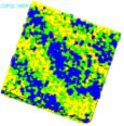
Taking the advantage of the multi-chain simulation, we have extended the PCN model into polymer blends and copolymers where the model is modified to take account the chemistry dependence in the parameters (unit time and unit length) and the interaction between the chemistries via the interaction parameter c. Figure 8 shows the coarsening process of lamellar structure of a block copolymer system where for simplicity all parameters of the two chemistries are the same, except for the interactions[14]. This kind of results has been frequently reported for the other simulation methods such like density functional simulations. However, it is noted that no other method can take account the effect of entanglement among polymers with practical computational cost.
Figure 8 Coarsening of lamellar structure for a block copolymer in PCN simulation
Multi-scale simulations for polymer processing
Utilizing the PCN simulation to predict the viscoelasticity of polymers, now we investigate the effect of molecular structure on macroscopic flow behavior. As an example, we performed a simulation of injection molding and examined the effect of molecular weight on warpage of the molded product [15]. I utilized the primitive chain network simulation to calculate linear viscoelasticity of linear monodispersed polystyrenes from molecular weight. The obtained linear viscoelasticity was converted into the relaxation spectrum and into the flow curve to be utilized in the macroscopic simulations. From the flow curve, the parameters of an inelastic non-Newtonian constitutive equation were obtained and used for the simulation of filling process. The relaxation spectrum was used to calculate residual stress from the flow profile in the filling process. From the residual stress and thermal shrinkage, warpage of the product was obtained. For the examined thin plate product, significant change in the warpage direction was demonstrated according to the molecular weight of the material.
Figure 9 Warpage prediction from molecular weight utilizing the PCN simulation
REFERENCES
- Ferry, J. D., Viscoelastic Properties of Polymers, 3rd ed., Wiley, New York, 1980
- Tadmor, Z.; Gogos, C. G., Principles of Polymer Processing, 2nd ed., Wiley, Hoboken, 2006
- Doi, M.; Edwards, S. F., The Theory of Polymer Dynamics, Clarendon, Oxford, 1986
- McLeish, T. C. B.; Larson, R. G., J. Rheol., 1998, 42, 81.; Likhtman, A. E.; Graham, R. S., J. Non-Newtonian Fluid Mech., 2003, 114, 1.
- Kremer K.; Grest, G. S., J. Chem. Phys., 1990, 92, 5057.
- Likhtman, A. E.; Sukumaran S. K.; Ramirez, J., Macromolecules, 2007, 40, 6748.
- Masubuchi, Y.; Takimoto, J.-I.; Koyama, K.; Ianniruberto, G.; Marrucci G.; Greco, F., J. Chem. Phys., 2001, 115, 4387.
- Masubuchi, Y.; Ianniruberto, G.; Greco F.; Marrucci, G., J. Non-Newtonian Fluid Mech., 2008, 149, 87.
- Masubuchi, Y.; Ianniruberto, G.; Greco F.; Marrucci, G., J. Chem. Phys., 2003, 119, 6925.
- Masubuchi, Y.; Watanabe H.; Ianniruberto, G.; Greco F.; Marrucci, G., Macromolecules, 2008, 41, 8275.
- Masubuchi, Y.; Ianniruberto, G.; Greco F.; Marrucci, G., Modelling Simul. Mater. Sci. Eng., 2004, 12, S91.
- Masubuchi, Y.; Ianniruberto, G.; Greco F.; Marrucci, G., Rheol. Acta, 2006, 46, 297.
- Masubuchi, Y.; Yaoita, T.; Matsumiya ,Y.; Watanabe, H.; Rheologica Acta, 2011, online publication.
- Masubuchi, Y.; Ianniruberto, G.; Greco F.; Marrucci, G., J. Non-Crystal. Solids, 2006, 352, 5001.
- Masubuchi, Y.; Uneyama, T; Saito, K.; J. Appl. Polym. Sci., in print.
*More papers on NAPLES can be found "here".